
This paper is available on arxiv under CC 4.0 license.
Authors:
(1) HARRISON WINCH, Department of Astronomy & Astrophysics, University of Toronto and Dunlap Institute for Astronomy and Astrophysics, University of Toronto;
(2) RENEE´ HLOZEK, Department of Astronomy & Astrophysics, University of Toronto and Dunlap Institute for Astronomy and Astrophysics, University of Toronto;
(3) DAVID J. E. MARSH, Theoretical Particle Physics and Cosmology, King’s College London;
(4) DANIEL GRIN, Haverford College;
(5) KEIR K. ROGERS, Dunlap Institute for Astronomy and Astrophysics, University of Toronto.
Table of Links
- Abstract and Intro
- Methods
- Phenomenology
- Discussion and Future Work
- Conclusion
- Acknowledgments and References
2. METHODS
In order to model the behavior of extreme axions, we modified axionCAMB to include an arbitrary field potential shape (in our case, a cosine of the form given in Equation 1), and reconfigured the code to sample the extreme starting angles necessary to probe these potentials. We also modified the effective sound speed of the axions after the onset of oscillations to reflect the growth in structure resulting from the tachyonic field dynamics. Lastly, we implemented a computationally-efficient ‘lookup table’ of the axion background fluid evolution in order to speed up the computation of the perturbation equations of motion. The details of implementing extreme axions into axionCAMB are presented below [2].
2.1. Review of axionCAMB
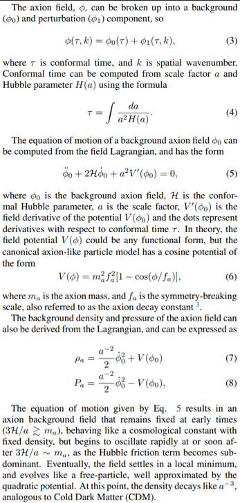
The numerical treatment of axions in axionCAMB is described in detail in Hlozek et al. ˇ (2015), but we review the dynamics of axions here in a potential-agnostic way in order to set up our discussion of modeling extreme axions. In theory, the best way of modeling the dynamics of axion dark matter is to model the behaviour of the field throughout all of cosmic history, and derive all cosmological parameters from those primary variables. However, since this field evolution includes periods of extremely rapid oscillations at late times, simulating this is computationally prohibitive and numerically unstable. Instead, the axion field is modeled directly at early times, but the code switches to a simplified fluid approximation at late times (Hlozek et al. ˇ 2015). This piecewise background evolution could then be called when solving the equations of motion for the fluid perturbations (axion density perturbation δa and axion heat flux u), allowing for efficient and stable computation of the final axion power spectrum. This method is discussed here, building on the discussion in Hu (1998) and Hlozek et al. ˇ (2015).
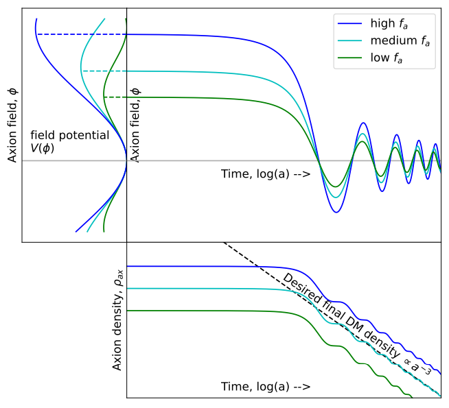
axionCAMB runs through this early pre-oscillatory phase several times in order to determine the proper initial value of the axion field required to produce the desired final axion density, and the time at which it can safely switch back to the free particle CDM solution at late times. It then dynamically evolves these initial conditions (integrating the equation of motion for a field using a Runge-Kutta integrator, Runge 1895) until the field starts to oscillate, at which point it switches over to the known free-particle solution for DM evolution (Hlozek et al. ˇ 2015).
This results in a new set of equations of motion for the axion perturbations after the onset of oscillations:
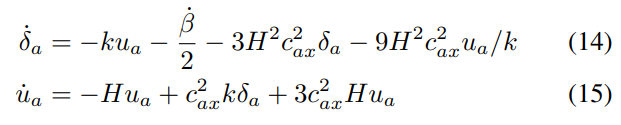
The perturbation equations of motion in these two regimes can be used to calculate the evolution of the axion perturbations, and make predictions for cosmological observables such as the MPS or CMB.
2.2. Finely tuned initial conditions
Restructuring the initial shooting methods to specify the field starting angle allows us to probe the effects of extreme starting angles in new ways. We can specify starting angles arbitrarily close to π, in order to see the effects of these extremely finely tuned angles on other observables. In addition, when performing MCMC analysis, having the starting angle as a free parameter allows us to impose arbitrary priors on this starting angle. We can use these priors to test the dependence of any constraints on the level of fine tuning of the axion starting angle.
2.3. Modeling the early-oscillatory effective axion sound speed
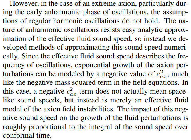
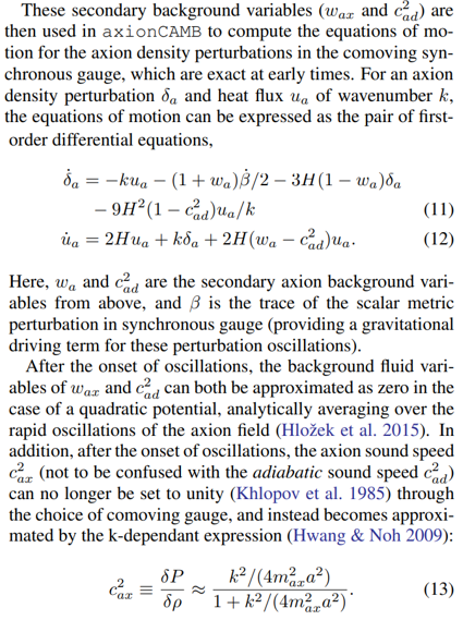
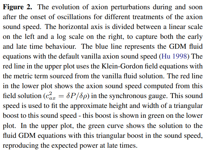
To get a sense of the effects of the anharmonic potential on the axion fluid sound speed, we first solve the axion field perturbation equations of motion,
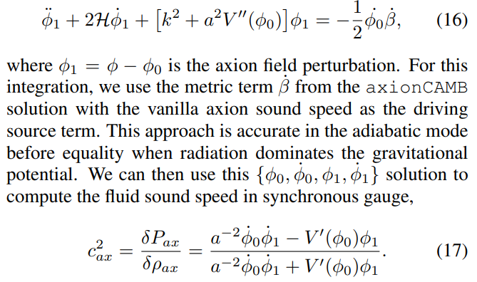
This approximation of the fluid sound speed is shown in red in the lower subplot of Figure 2.
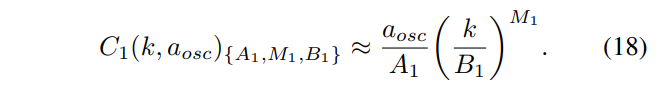
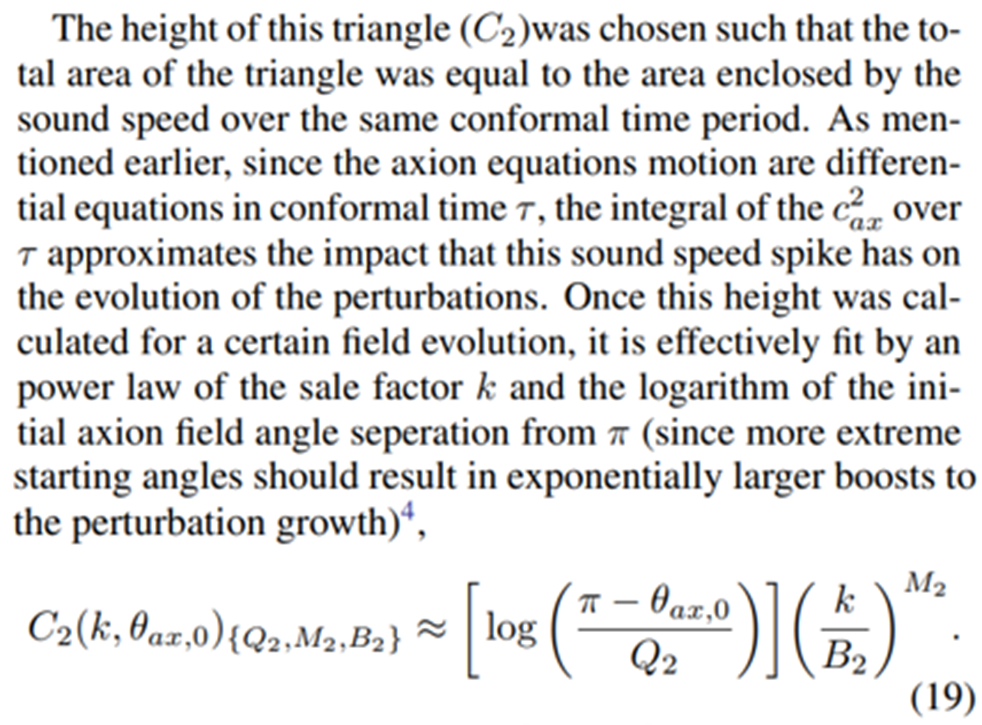
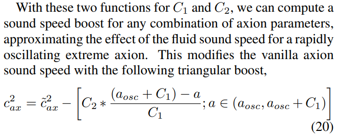
In order to approximate the boost in the axion sound speed shown in the field equations without changing the late-time evolution of the perturbations, we modified the vanilla axion fluid sound speed to include a large negative spike just after the onset of oscillations. This negative triangular spike is shown in green in the lower subplot of Figure 2. The width and height of this spike were fit to match the approximate sound speed computed from the field perturbation solution. The width (C1) was fit to the delay in scale factor a between the onset of axion oscillations and the asymptotic sign change in the field solution sound speed. This numerical width was then approximated as a power law function of the scale factor k of the perturbation, depends linearly on the scale factor at the onset of oscillations, which in turn depends on the axion mass, fraction, and starting angle,
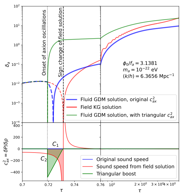
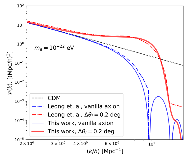
The power spectrum results for this method can be compared to the literature, where other groups have used the exact field perturbation equations of motion to compute the matter power spectrum for extreme axions, such as Leong et al. (2019). In Figure 3 we can see the comparison in the matter power spectrum for both a vanilla axion and an extreme axion with a starting angle deviating from π by 0.2 degrees, and we find that they are in remarkably close agreement with Leong et al. (2019). However, this close agreement seems to hold best at z = 0, when these power spectra are computed, while the higher redshifts comparison may be more nuanced. Figure 2 suggests that while the exact field solution and the new approximate fluid solution agree at very late times, their evolution at early times are not fully equivalent, so more work may need to be done on this approximation in order to perform comparisons to high-redshift observables.
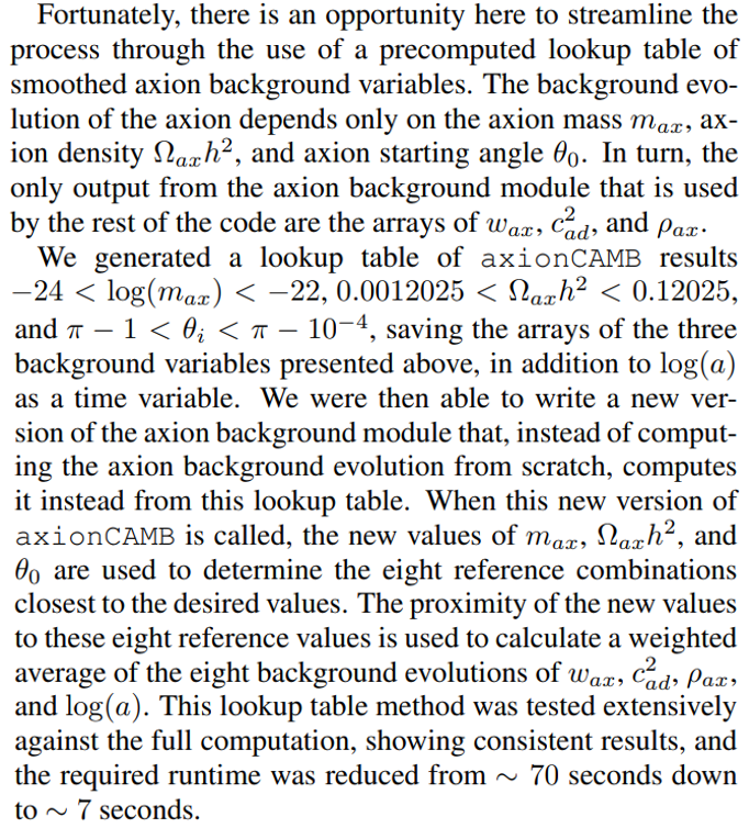
2.4. Using lookup tables for efficient modeling of field
Extending the full field evolution so much later past the onset of oscillations requires far more computational resources than ending the field evolution as soon as oscillations begin. Greater numerical resolution, in both time and possible field potential scale, is also required to integrate these rapidly oscillating variables. With these increases to computational time, the new version of axionCAMB takes around seventy seconds to complete. While this may be feasible when computing a single power spectrum result, this is computationally intensive with which to run an MCMC analysis, which may require tens to hundreds of thousands of separate calls to axionCAMB.
2.5. Summary of changes to axionCAMB
In order to model axions with extreme starting angles in a cosine field potential using the computationally efficient field formalism used in axionCAMB, we have introduced a number of modifications to axionCAMB which are explained above, but summarized here.
• We replaced the quadratic approximation of the field potential with an arbitrary potential function, currently set to the canonical cosine potential.
• We modified the effective axion fluid sound speed to reproduce the growth in structure seen in the exact field perturbation equations of motion.
• We precomputed a lookup table for the axion background evolution which significantly reduced the runtime.
The result is an accurate modeling of extreme axion background and perturbation evolution for an arbitrary axion mass, density, and starting angle that only takes ∼ 7 seconds to run. This powerful tool can shed new light on the behaviour and detectability of these extreme axion models, as discussed below.
2.6. Data: Ly-α forest estimates of the MPS
[2] axionCAMB is in turn based on the cosmological Boltzmann code, CAMB (Lewis & Bridle 2002).
[4] A logarithmic dependence for the background field can be derived analytically for the anharmonic corrections to the relic density (Lyth 1992).