This paper is available on arxiv under CC 4.0 license.
Authors:
(1) Z. Jennings, Astrophysics Group, Keele University, Staffordshire, ST5 5BG, UK (E-mail: z.jennings@keele.ac.uk);
(2) J. Southworth, Astrophysics Group, Keele University, Staffordshire, ST5 5BG, UK;
(3) K. Pavlovski, Department of Physics, Faculty of Science, University of Zagreb, 10000 Zagreb, Croatia;
(4) T. Van Reeth, Institute of Astronomy, KU Leuven, Celestijnenlaan 200D, B-3001 Leuven, Belgium.
Table of Links
- Abstract and Intro
- Observation
- Orbital Ephemeris
- Radial Velocity Analysis
- Spectral Analysis
- Analysis of the Light Curve
- Physical Properties
- Asteroseismic Analysis
- Discussion
- Conclusion, Data Availability, Acknowledgments, and References
- Appendix A: Ephemeris Determination
- Appendix B: Iteratively Prewhitened Frequencies
- Appendix C: Detected Tidally Perturbed Pulsations
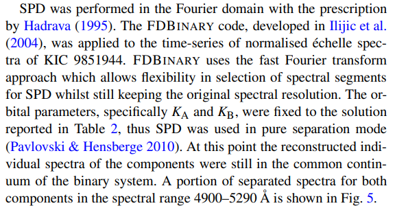
5 SPECTRAL ANALYSIS
5.1 Atmospheric parameters
Since we planned to apply the method of SPD to extract the individual spectra of the components, normalisation of the observed spectra was of critical importance. We used a different approach than that in Section 4, where we extracted RVs. Here, we used the dedicated code described in Kolbas et al. (2015). First, the blaze function of échelle orders was fitted with a high-order polynomial function. Then, the normalised échelle orders were merged. When overlapping regions of successive échelle orders are sufficiently long, the very ends were cut off because of their low S/N. Échelle orders containing broad Balmer lines, in which it is not possible to define the blaze function with enough precision, were treated in a special way. For these échelle orders, the blaze function was interpolated from adjacent orders. This produces more reliable normalisation in spectral regions with broad Balmer lines than the usual pipeline procedures. For recent applications of this approach, please see Pavlovski et al. (2018, 2023); Lester et al. (2019, 2022); Wang et al. (2020, 2023).
Overall, a slight difference in line depth between the two components is seen. The more massive component has deeper lines and slightly faster rotation. The Balmer lines are broadened by Stark broadening, and generally are not sensitive to the rotational broadening. Thus, we first optimised portions of the disentangled spectra free of the Balmer lines, primarily to discern the vsini values. We then performed optimal fitting of disentangled spectra centred on the Hβ and Hα lines, with fixed vsini.

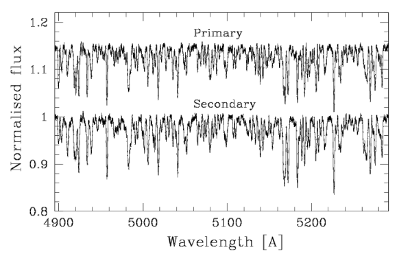
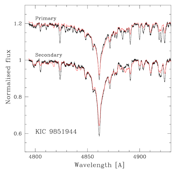
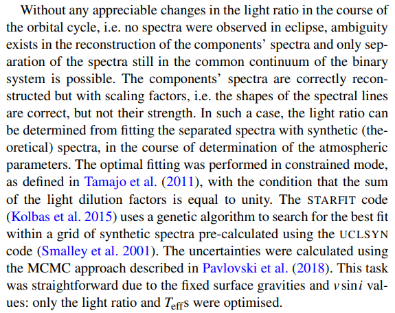
The light ratio from the optimal fitting of the wings of Hβ and Hγ lines, spectral segments containing only metal lines, and the Mg I triplet at around 5180 Å, are 1.315±0.018, 1.304±0.025 and 1.278±0.033 (Table 3). All three values for the light ratio are consistent within their 1σ uncertainties, with the light ratio determined from the wings of Hβ line being the most precise of the three.
Guo et al. (2016) determined atmospheric parameters from tomographically reconstructed spectra of the components. Their spectra cover the wavelength range 3930–4610 Å at a medium spectral resolution of R = 6000. The analysis by Guo et al. (2016) was similar to ours, but with an important difference that they fitted complete separated spectra, whilst we concentrate on the wings of Balmer lines. Our results for the Balmer lines corroborate their findings to within 1σ. We also find good agreement for the vsini values, which are also within 1σ for both components. Guo et al. (2016) obtained a mean light ratio 1.34±0.03 from spectra centred at 4275 Å – this is slightly larger than but still consistent with our own results.
5.2 Direct fitting for the light ratio
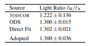
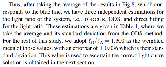
We were initially unable to constrain the light ratio of the system from the photometric analysis alone (see Section 3), so estimated it using several independent methods. The first method was the TODCOR light ratio reported in Table 2, the second was the optimal fitting of the disentangled spectra (ODS), and a third method is developed here.
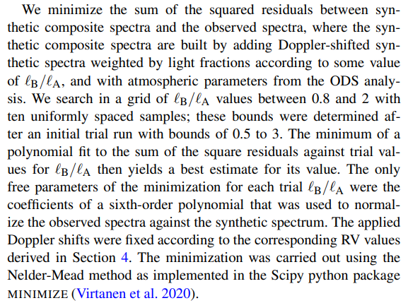
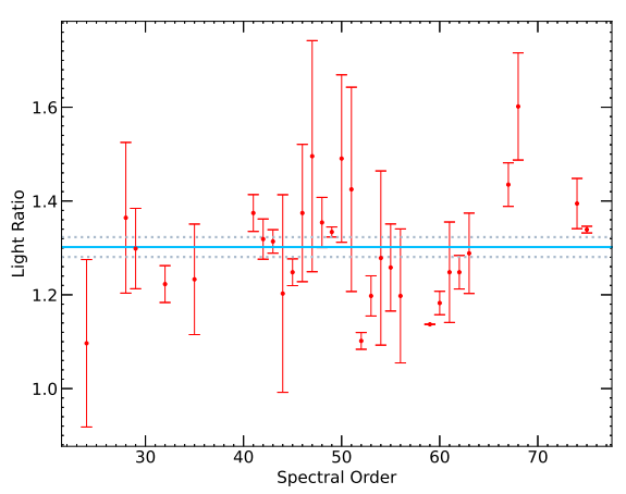
We repeated the process for all spectral orders showing sufficient well-resolved lines in regions unaffected by tellurics from Earth’s atmosphere. To save computing time, only the two observations closest to positions of quadrature were used. This approach resulted 036 30 spectral orders showing adequate fits with well defined minima in the sum of the square residuals. Fig.7 shows the result of this method applied to order 66, which demonstrates the effectiveness of optimizing the normalization of the observed spectra in the fitting routine for an order where line blending is significant. The resulting values for ℓB/ℓA after applying this method to the selected orders are shown in Fig.8, where each result is the average of the result from each of the two observations used.